Build your own ChatGPT from scratch in Python numpy

Generative Pre-trained Transformers, or GPTs, represent a significant leap forward in natural language processing technology. These models, especially notable ones like OpenAI’s GPT-3, are celebrated for producing text that is not only fluent but also contextually aware, marking a new era in our engagement with AI-driven language models. But constructing a GPT model involves what specific processes? We shall explore the intricacies of Transformer technology and outline the steps to assemble a GPT from the ground up using Python and NumPy.

GPTs are distinguished by their vast network size, with some housing billions of parameters and being honed on wide-ranging datasets. This immense size equips them to handle diverse linguistic tasks, ranging from composing emails to distilling intricate ideas into accessible language.

In embarking on the journey to craft a GPT model using Python and NumPy, it’s crucial to grasp the architecture’s underlying elements and their synergy, particularly within the sphere of NLP. We will delve into these fundamental concepts and offer an in-depth breakdown of each aspect to forge an exhaustive tutorial.

Step 1: Setting Up the Environment

First, clone the necessary repository and set up the environment:

GitHub — jaymody/picoGPT: An unnecessarily tiny implementation of GPT-2 in NumPy.

import numpy as np
import sys
!git clone https://github.com/jaymody/picoGPT.git
# Pretrained weights are from https://github.com/jaymody/picoGPT
sys.path.append('./picoGPT')

Step 2: Defining Basic Functions

The building blocks of our GPT are functions like GELU (Gaussian Error Linear Unit), linear layers, softmax, and layer_norm mechanisms:

def gelu(x):
    # GELU activation function applies a non-linear activation to the input 'x'
    # It's used to introduce nonlinearity in the model and helps with learning complex patterns
    return 0.5 * x * (1 + np.tanh(np.sqrt(2 / np.pi) 
                                  * (x + 0.044715 * x**3)))
def linear(x, w, b):
    # Linear transformation function that computes the weighted sum of the inputs 'x' plus a bias 'b'
    # 'w' are the weights and 'b' is the bias term, this is a basic building block of neural networks
    return x @ w + b

def softmax(x):
    exp_x = np.exp(x - np.max(x, axis=-1, keepdims=True))
    return exp_x / np.sum(exp_x, axis=-1, keepdims=True)

def ffn(x, c_fc, c_proj):
    a = gelu(linear(x, **c_fc))
    x = linear(a, **c_proj)
    return x

def layer_norm(x, g, b, eps: float = 1e-5):
    # Feedforward network function that applies a GELU activation after a linear transformation
    # followed by another linear transformation
    # It's a sequence of operations commonly used in transformers
    mean = np.mean(x, axis=-1, keepdims=True)
    variance = np.var(x, axis=-1, keepdims=True)
    x = (x - mean) / np.sqrt(variance + eps)
    return g * x + b

2.1 GELU vs other activefunction

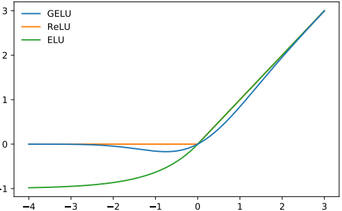
GPT employs GELU (Gaussian Error Linear Unit) as its activation function due to its superior performance demonstrated in practice. GELU is a relatively new type of activation function introduced by Hendrycks and Gimpel in 2016. It incorporates characteristics of the ReLU (Rectified Linear Unit) and the probability distribution properties of the normal distribution. The specific expression for the GELU function is:

Some advantages of GELU include:

• Non-saturating: GELU provides non-linear activation, but unlike ReLU, it is not entirely saturated for negative values, which helps with the flow of gradients and reduces the problem of vanishing gradients.
• Smooth Gradients: Due to its smooth nature, GELU can provide continuous gradients, which contributes to stability and performance during the training process.
• Probabilistic Interpretation: Since it emulates the “gating” of input values (i.e., the probabilistic weight of the input value x), it introduces a degree of natural randomness, which can help with regularization of the model and potentially improve its generalization ability.
• Empirical Performance: GELU has shown better performance than other activation functions across various tasks and benchmarks. Particularly in NLP tasks, the combination of GELU with the Transformer model has proven to be highly effective.

2.2 Softmax implementation

We can observe that there are certain differences between the softmax function’s theoretical formula and its implementation in code.

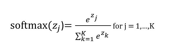
Modifications have been made to the softmax computation within the code, primarily to enhance numerical stability.

def softmax(x):
    exp_x = np.exp(x - np.max(x, axis=-1, keepdims=True))
    return exp_x / np.sum(exp_x, axis=-1, keepdims=True)

• Overflow and Underflow: Direct computation of exp(x_i) can be problematic because the exponentiation can result in very large numbers for moderate values of x_i (overflow) or very small numbers for large negative values of x_i (underflow), leading to numerical instability. Subtracting the max value np.max(x) from each element in x before exponentiation helps to mitigate this risk because the largest value in the adjusted vector will be 0, which, when exponentiated, equals 1. This subtraction makes the largest of the exp values 1, preventing overflow in the numerator and denominator.
• Numerical Stability: By normalizing the values (shifting the inputs to a smaller range), the softmax function becomes more numerically stable. Without this step, the computation of exp(x_i) for large x_i could result in an infinite value in floating-point arithmetic, which would lead to NaN values during division.
• Efficiency: The use of axis=-1 and keepdims=True allows the function to be applied to multi-dimensional arrays and maintain their shape, which is useful when computing softmax across certain dimensions (like batches of data or different features) in more complex models.

2.3 LayerNorm vs BatchNorm

Layer Normalization (LayerNorm) and Batch Normalization (BatchNorm) are both techniques used to stabilize and accelerate the training of deep neural networks, but they work in slightly different ways and are used in different contexts.

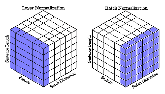
Here’s a comparison:

Batch Normalization (BatchNorm):

• Normalizes the output of a previous activation layer by subtracting the batch mean and dividing by the batch standard deviation (hence the name “batch” normalization).
• The normalization is done over the batch dimension, i.e., for each feature, BN computes the mean and variance over the batch of data.
• It is typically applied to the inputs of the activation function in a layer.
• BatchNorm has parameters (scale and shift) that are learnable during training. It requires a sufficiently large batch size to work well since the statistics are computed over the batch.
• It can lead to significant improvements in convergence for convolutional neural networks (CNNs) and fully connected layers.

Layer Normalization (LayerNorm):

• Normalizes the inputs across the features instead of the batch. For each data point in the batch, LayerNorm computes the mean and variance used for normalization across the features.
• It is particularly useful in recurrent neural networks (RNNs) and Transformer models, where the batch size can often be one, or the sequence length can vary.
• LayerNorm also has learnable parameters (gain and bias) that can be adjusted during training. Since LayerNorm does not rely on the batch dimension, it behaves consistently during training and inference.
• It has been found to be more effective than BatchNorm in sequence models where the temporal dynamic is important, as it normalizes across the features at each time step.

In summary, BatchNorm is effective for tasks where the batch size is large and consistent, and it’s commonly used in CNNs. LayerNorm, on the other hand, is more suited to sequence models like RNNs and Transformers because it doesn’t depend on batch statistics and therefore can handle variable sequence lengths and smaller batch sizes.

Step 3: Implementing Multi-Head Attention and Feed-Forward Networks

Multi-head attention and feed-forward networks are crucial for the model:

def attention(q, k, v, mask):
    s = q @ k.T
    s = s / np.sqrt(q.shape[-1]) + mask
    p = softmax(s)
    o = p @ v
    return o

# Multi-head attention
def mha(x, c_attn, c_proj, n_head):
    x = linear(x, **c_attn)
    qkv = np.split(x, 3, axis=-1)
    qkv_heads = list(map(lambda x : np.split(x, n_head, axis=-1), qkv))
    
    causal_mask = (1 - np.tri(x.shape[0], dtype=x.dtype)) * -1e10
    out_heads = [attention(q,k,v, causal_mask) for q, k, v in zip(*qkv_heads)]
    x = np.hstack(out_heads)
    x = linear(x, **c_proj)
    return x

The foundation of GPT lies in the Transformer model, a type of deep learning model designed to handle sequential data like text.

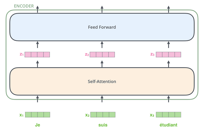
Self-attention Mechanism: This allows the model to weigh the importance of different words in a sentence, providing a dynamic understanding of textual context.

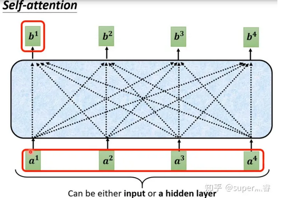
Imagine you’re reading a complex novel, and in each sentence, some words are more important to the meaning than others. For instance, in the sentence “The cat sat on the mat,” words like “cat” and “mat” are more crucial to understanding the sentence than “the” or “on.” Self-attention in a neural network works similarly. It helps the model to focus more on certain words (or parts of the input) when trying to understand or generate text.

In essence, self-attention is like a smart, dynamic highlighter that helps AI models determine which words in a sentence are the most important for understanding the meaning and context, much like how we focus on certain words while reading or listening to make sense of the information.

Here, for each word, we have k, v, q; k and v represent the associations between them. In the self-attention mechanism, “K,” “Q,” and “V” stand for “Key,” “Query,” and “Value,” respectively. These terms come from the field of information retrieval and are used to help the model determine how much attention to give to a given input, such as a word or phrase. Here’s how they work:

• Query: The query represents the current word or item being considered, which can be thought of as a search query looking for other related information.
• Key: The key corresponds to the representation of all other words or items in the database, which can be imagined as index keywords used by the query to find matching items.
• Value: Once a query finds a matching item through a key, the associated value is used to calculate a new representation of the input word or item. The value contains the actual information you want to retain in the output of the attention mechanism.

In the self-attention mechanism, each input element, such as a word, is transformed into representations of query, key, and value. The model allocates attention scores by calculating the compatibility between the query and all keys, typically done by taking their dot product and then applying the softmax function to ensure that all attention scores add up to 1. These scores are then used to weight the corresponding values, resulting in the final output representation of each input element. This output captures the context information of all elements in the input sequence.

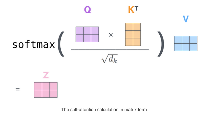
In fact, matrix operations are used in the implementation:

• Efficiency: Matrix operations can efficiently utilize modern hardware architectures, especially GPUs (Graphics Processing Units) and TPUs (Tensor Processing Units), which are designed for large-scale parallel computations. Converting the calculations of the attention mechanism into matrix operations can significantly speed up training and inference processes.
• Batch Processing: Matrix operations allow us to process multiple data samples simultaneously, known as batch processing. This means that the network can learn from multiple examples at once, making more effective use of computational resources.
• Vectorization: Matrix and vectorized computations reduce the number of necessary iterations, eliminating the need for explicit loops for each operation. This not only simplifies the complexity of writing code but also reduces computation time.

Step 4: Building the Transformer Blocks

Each transformer block in GPT consists of multi-head attention and feed-forward networks, along with layer normalization:

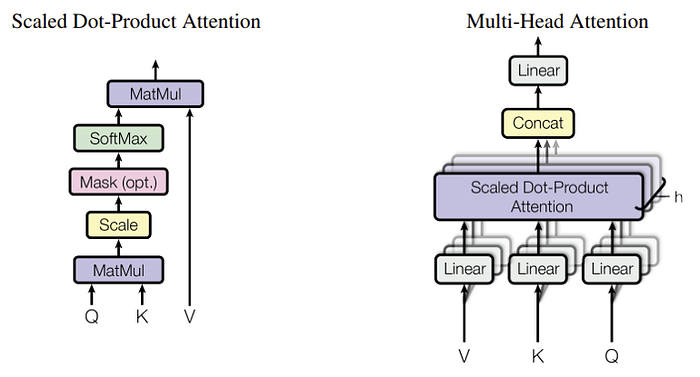
def transformer_block(x, mlp, attn, ln_1, ln_2, n_head):
    x = x + mha(layer_norm(x, **ln_1), **attn, n_head=n_head)
    x = x + ffn(layer_norm(x, **ln_2), **mlp)
    return x

Step 5: Assembling the GPT Model

Now, we assemble these components to create the GPT model:

GPT is built upon the Transformer architecture, focusing on the decoder part for text generation.

• Decoder Blocks: These are the building blocks of GPT. Each block includes a self-attention layer followed by a feed-forward neural network.
• Layer Normalization and Skip Connections: These components help in stabilizing the learning process and enabling the training of deep networks.

def gpt2(inputs, wte, wpe, blocks, ln_f, n_head):
    x = wte[inputs] + wpe[range(len(inputs))]
    for block in blocks:
        x = transformer_block(x, **block, n_head=n_head)
    x = layer_norm(x, **ln_f)
    return x @ wte.T

Step 6: Generating Text

The process of generating text in GPT involves predicting the next word in a sequence given the previous words.

• Tokenization: The input text is broken into tokens (words or subwords) which are then converted into numerical representations.
• Predictive Modeling: The model predicts the next token based on the previous tokens, using its learned understanding of language patterns.

To generate text, we use the model to predict the next token in a sequence iteratively:

def generate(inputs, params, n_head, n_tokens_to_generate):
    from tqdm import tqdm
    
    for _ in tqdm(range(n_tokens_to_generate), "generating"):
        logits = gpt2(inputs, **params, n_head=n_head)
        next_id = np.argmax(logits[-1])
        inputs.append(int(next_id))
    return inputs[len(inputs) - n_tokens_to_generate :]

Step 7: Running the Model

Finally, we create a function to run our model with a given prompt:

def main(prompt: str, n_tokens_to_generate: int = 40, 
         model_size: str = "124M", models_dir: str = "models"):
    from utils import load_encoder_hparams_and_params
    encoder, hparams, params = load_encoder_hparams_and_params(model_size, models_dir)
    input_ids = encoder.encode(prompt)
    
    assert len(input_ids) + n_tokens_to_generate < hparams["n_ctx"]
    
    output_ids = generate(input_ids, params, hparams["n_head"], n_tokens_to_generate)
    
    output_text = encoder.decode(output_ids)
    return output_text

main("What is LLM?")

2023-10-25 22:49:45.842762: I tensorflow/core/platform/cpu_feature_guard.cc:182] This TensorFlow binary is optimized to use available CPU instructions in performance-critical operations.
To enable the following instructions: SSE4.1 SSE4.2 AVX AVX2 FMA, in other operations, rebuild TensorFlow with the appropriate compiler flags.
Fetching checkpoint: 1.00kb [00:00, 6.07Mb/s]                                                       
Fetching encoder.json: 1.04Mb [00:00, 3.13Mb/s]                                                     
Fetching hparams.json: 1.00kb [00:00, 4.89Mb/s]                                                     
Fetching model.ckpt.data-00000-of-00001: 498Mb [00:22, 22.0Mb/s]                                    
Fetching model.ckpt.index: 6.00kb [00:00, 7.37Mb/s]                                                 
Fetching model.ckpt.meta: 472kb [00:00, 1.95Mb/s]                                                   
Fetching vocab.bpe: 457kb [00:00, 1.90Mb/s]                                                         
generating: 100%|████████████████████████████████████████████████████████████████████████████████████████████████████| 40/40 [00:02<00:00, 13.49it/s]

Now you can find you own GPT works~

'\n\nLLM is a programming language that is designed to be used in a variety of applications. It is a programming language that is designed to be used in a variety of applications. It is a'

Conclusions

In conclusion, constructing your own Generative Pre-trained Transformer (GPT) from scratch is a challenging yet incredibly rewarding endeavor that underscores the remarkable capabilities of Python and NumPy in the realm of natural language processing. Throughout this article, we have navigated the foundational elements of GPT architecture, from understanding the intricacies of self-attention and position encoding to grappling with the complexities of large-scale model training. The process reveals not just the technicalities of building a state-of-the-art language model but also illuminates the nuances of machine learning workflows and the importance of computational efficiency. Armed with the insights and methodologies discussed, one is well-equipped to embark on the journey of creating a custom GPT model, tailored to unique tasks and capable of pushing the boundaries of what we expect from AI in language understanding and generation. Whether for academic exploration, industry innovation, or personal projects, the knowledge to build a GPT model from scratch in Python using NumPy is a powerful tool in any developer’s arsenal.