Generative Modeling via Drifting: Training-Time Pushforward Evolution for One-Step Generation
Mingyang Deng, He Li, Tianhong Li, Yilun Du, and Kaiming He (MIT & Harvard, arXiv:2602.04770) introduce Drifting Models, moving iterative distribution evolution from inference time to training time. Driven by a kernelized attraction-repulsion drifting field in self-supervised feature space, a single-pass DiT-L generator reaches 1.54 FID in latent space and 1.61 FID in pixel space on ImageNet 256×256 at 1-NFE, while matching 100-step Diffusion Policy on robotic control.
Abstract and Core Findings
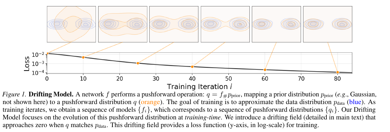
Generative models learn a mapping such that the pushforward distribution of a prior matches the data distribution: . Diffusion and Flow Matching models decompose this transport map into a chain of small steps executed at inference time through stochastic or ordinary differential equation (SDE/ODE) solvers. In Generative Modeling via Drifting (arXiv:2602.04770), Mingyang Deng, He Li, Tianhong Li, Yilun Du, and Kaiming He at MIT and Harvard University move the iterative evolution of the pushforward distribution entirely to training time.
Because neural network optimization already produces a sequence of parameters across training iterations, it induces a corresponding trajectory of pushforward distributions where . To steer toward , the authors define an anti-symmetric drifting field that pulls generated samples toward real data points (attraction) and pushes them away from other generated samples (repulsion). When , attraction and repulsion cancel out (), reaching a zero-drift equilibrium. At inference time, the trained network maps noise to data in a single non-iterative forward pass (1 neural function evaluation, or 1-NFE).
Four empirical results summarize the paper's contributions:
- State-of-the-art 1-NFE latent-space generation on ImageNet . Trained from scratch without distillation or SDE/ODE trajectory approximation,
Drifting Model L/2(463M generator parameters + 49M SD-VAE decoder parameters) achieves 1.54 FID and 258.9 IS in a single step at CFG scale . The smallerDrifting Model B/2(133M + 49M parameters) reaches 1.75 FID, outperforming 675M-parameter XL-scale single-step diffusion and flow models includingiCT-XL/2(34.24 FID),Shortcut-XL/2(10.60 FID),MeanFlow-XL/2(3.43 FID), andAdvFlow-XL/2(2.38 FID). - 1.61 FID in direct pixel-space 1-NFE generation at 18x lower compute than StyleGAN-XL. Operating directly on pixels without a latent VAE tokenizer,
Drifting Model L/16(464M parameters, 87G FLOPs) reaches 1.61 FID and 307.5 IS at 1-NFE. This surpasses prior single-step pixel-space flow models (EPG-L/16, 8.82 FID), pixel-space GANs (StyleGAN-XL, 2.30 FID at 1574G FLOPs;GigaGAN, 3.45 FID), and multi-step pixel-space diffusion models such asADM-G(4.59 FID at NFE) andJiT-G/16(1.82 FID at NFE). - Strict necessity of anti-symmetry for distribution equilibrium. In controlled ImageNet ablations (
DiT-B/2, 100 epochs), the balanced anti-symmetric field achieves 8.46 FID. Perturbing the balance to or degrades FID to 41.05 and 46.28, and removing repulsion ( only) collapses generation to 177.14 FID. - Drop-in 1-NFE replacement for 100-NFE Diffusion Policy in robotics control. Replacing the 100-step diffusion generator in Diffusion Policy with a 1-NFE Drifting Policy operating directly on raw state or visual action representations matches or improves task success rates across
Lift(1.00),Can(0.99),ToolHang(0.67 visual / 0.38 state),PushT(0.86),BlockPush(0.56 Phase 1 / 0.16 Phase 2 vs. 0.36 / 0.11 for 100-NFE Diffusion Policy), andKitchen(0.96 Phase 4).
1. Pushforward Evolution at Training Time and the Zero-Drift Equilibrium
Let be a neural network mapping prior noise to generated samples . In probability theory, is the pushforward distribution of under . Every parameter update during stochastic gradient descent shifts the generated sample for a given noise input by a residual , evolving the pushforward distribution from to .
To govern this training-time sample movement explicitly, Deng et al. introduce a drifting field parameterized by the target distribution and the current generated distribution :
Proposition 3.1 (Anti-Symmetric Equilibrium). If the drifting field is anti-symmetric with respect to and , meaning
then matching the distributions guarantees zero drift everywhere:
At the equilibrium parameter where , the generator satisfies the fixed-point relation . Turning this fixed-point iteration into a tractable neural network objective without backpropagating through the distribution yields the stop-gradient regression loss:
At each iteration, the target is frozen. Two mathematical properties follow directly from this formulation:
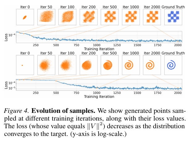
- Exact Drift Norm Value: The scalar value of evaluated at iteration is identically , providing a direct quantitative monitor of how close the system is to equilibrium.
- Direct Gradient Equivalence: Differentiating with respect to gives , so parameter gradients follow without computing higher-order derivatives of .
2. Kernelized Mean-Shift Attraction and Repulsion
To instantiate an anti-symmetric field , the authors draw inspiration from Mean-Shift mode seeking (Cheng, 1995) and contrastive representation learning (InfoNCE). They define an attraction vector weighted by positive real samples and a repulsion vector weighted by negative generated samples :
where the partition functions and normalize the similarity kernel at temperature .
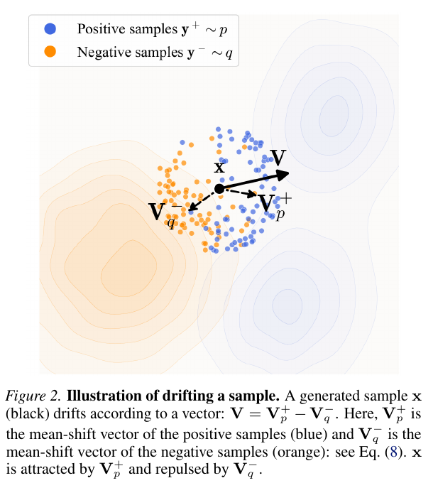
Subtracting repulsion from attraction yields the combined drifting field:
Because swapping and exchanges and , the vector difference changes sign while the product remains invariant, satisfying Proposition 3.1 ().
2.1 Why Doubly-Normalized Kernels Succeed Where Unnormalized MMD Fails
In Appendix C.2, the authors prove that classical Maximum Mean Discrepancy () with a radial kernel induces an unnormalized drifting field where . In high-dimensional spaces, unnormalized Gaussian kernels suffer from kernel vanishing when samples are far apart, and the authors report that unnormalized MMD fails to train competitive ImageNet generators.
Drifting Models resolve this by implementing as a softmax operation over the batch of positive and negative samples, combined with a second softmax normalization across the batch of query samples (Algorithm 2):
# x: [N, D] generated samples; y_pos: [N_pos, D] real samples; y_neg: [N_neg, D] negatives
dist_pos = cdist(x, y_pos)                  # [N, N_pos] pairwise L2 distances
dist_neg = cdist(x, y_neg) + eye(N) * 1e6   # [N, N_neg] mask out self-similarity
logit = cat([-dist_pos / T, -dist_neg / T], dim=1)

# Doubly-stochastic geometric mean normalization across rows (y) and columns (x)
A_row = logit.softmax(dim=-1)
A_col = logit.softmax(dim=-2)
A = sqrt(A_row * A_col)

A_pos, A_neg = split(A, [N_pos], dim=1)
W_pos = A_pos * A_neg.sum(dim=1, keepdim=True)
W_neg = A_neg * A_pos.sum(dim=1, keepdim=True)

V = (W_pos @ y_pos) - (W_neg @ y_neg)
x_drifted = stopgrad(x + V)
loss = mse_loss(x - x_drifted)
2.2 Toy Distribution Evolution and Resistance to Mode Collapse
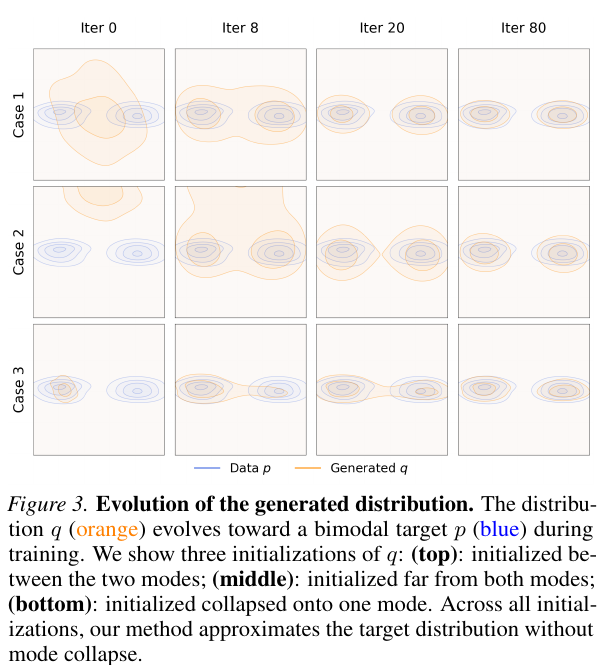
Figures 3 and 4 illustrate how this attraction-repulsion dynamics avoids mode collapse on 2D multimodal targets. Even when the generator distribution is initialized completely collapsed onto a single mode of a bimodal target (Figure 3, Case 3), repulsion among the crowded generated samples and uncompensated attraction from the unoccupied second mode pull mass across the gap until both modes are covered equally.
3. Multi-Scale Self-Supervised Feature Drifting and Training-Time CFG
Raw pixel or VAE-latent distances poorly reflect semantic similarity on complex natural datasets like ImageNet; in raw latent space without a feature encoder, the kernel becomes nearly flat. Deng et al. therefore compute the drifting field across multi-scale, multi-location feature maps extracted from a frozen, pre-trained self-supervised image encoder :
Crucially, the feature encoder is only evaluated during training. At inference time, the generator produces latent codes or pixels directly in 1-NFE without running .
3.1 Scale-Invariant Feature and Drift Normalization
For a ResNet-style encoder with 4 stages at spatial resolutions and channel widths , the authors extract per-location vectors, global means and standard deviations, and / patch means and standard deviations from every two residual blocks. To combine hundreds of feature losses without manual per-layer weighting, two parameter-free normalizations are applied at each feature index (dimension ):
- Feature Distance Normalization (): Features are scaled by with so that the expected pairwise distance equals . Setting the effective kernel temperature to makes invariant to both feature magnitude and channel dimensionality. The authors sum the normalized drifts over three fixed temperatures before computing the MSE loss.
- Unit-Variance Drift Normalization (): Each aggregated drift vector is scaled by where , ensuring across all spatial scales.
3.2 Training-Time Classifier-Free Guidance (CFG)
Standard diffusion CFG requires two network evaluations per step at inference time (conditional and unconditional). Drifting Models bake CFG into the training-time negative distribution while keeping inference strictly 1-NFE. Given class condition , positive samples are drawn from , while negative samples are drawn from a mixture of generated conditional samples and unconditional real data samples :
Enforcing the equilibrium condition solves for the learned generator distribution:
During training, is sampled per class following a power-law distribution (or ) and passed to the DiT generator via adaLN-zero conditioning alongside 16 in-context register tokens and 32 StyleGAN-inspired random codebook style tokens. At inference time, any guidance scale can be specified in a single forward pass.
4. Empirical Ablations on ImageNet
All baseline ablations use a DiT-B/2 generator (133M parameters) operating on SD-VAE latents, trained for 100 epochs with effective batch size and evaluated via FID-50K.
4.1 Destructive Study of Anti-Symmetry and Sample Allocation
Breaking the anti-symmetric balance immediately destroys generation fidelity (Table 1 of the paper), while scaling both and under a fixed 4096 batch budget steadily reduces FID by reducing Monte Carlo variance in the empirical drift estimate (Table 2):
| Study Dimension | Configuration / Field Definition | 1-NFE FID () | |
|---|---|---|---|
| Anti-Symmetry (Default) | (Exact equilibrium when ) | 8.46 | |
| 1.5x Attraction Bias | 41.05 | ||
| 1.5x Repulsion Bias | 46.28 | ||
| 2.0x Attraction Bias | 86.16 | ||
| 2.0x Repulsion Bias | 112.84 | ||
| Attraction Only | (No repulsion among generated samples) | 177.14 | |
| Positive Sample Scaling | (fixed ) | $20.43 \to 10.39 \to 8.97 \to \mathbf{8.46}$ | |
| Negative Sample Scaling | (fixed ) | $11.82 \to 10.16 \to 9.32 \to \mathbf{8.46}$ |
4.2 Feature Encoder Quality (SimCLR, MoCo-v2, and latent-MAE)
Standard pixel-space self-supervised ResNet-50 encoders (SimCLR and MoCo-v2) work out of the box when gradients are backpropagated through the SD-VAE decoder, reaching 11.05 and 8.41 FID respectively. To avoid running the VAE decoder during latent-space training, the authors pre-train a multi-scale ResNet-34 with GroupNorm directly on latents using a 50% patch-zeroing Masked Autoencoder (latent-MAE) objective:
| Feature Encoder () | Architecture & Block | Base Width | SSL Pre-Train Epochs | 1-NFE FID (, B/2 100 ep) |
|---|---|---|---|---|
SimCLR |
ResNet-50 (bottleneck, pixel) | 256 | 800 | 11.05 |
MoCo-v2 |
ResNet-50 (bottleneck, pixel) | 256 | 800 | 8.41 |
latent-MAE (Default) |
ResNet-34 (basic, latent) | 256 | 192 | 8.46 |
latent-MAE (Wider) |
ResNet-34 (basic, latent) | 384 / 512 / 640 | 192 | 7.26 / 6.49 / 6.30 |
latent-MAE (Longer SSL) |
ResNet-34 (basic, latent) | 640 | 1280 | 4.28 |
latent-MAE + cls ft |
ResNet-34 (basic, latent + 3k linear cls fine-tune) | 640 | 1280 | 3.36 |
Scaling the DiT-B/2 generator with the latent-MAE + cls ft encoder from 100 epochs (3.36 FID) to 320 epochs reduces FID to 2.51, and training for 1280 epochs with batch size reaches 1.75 FID. Scaling the generator backbone to DiT-L/2 (24 layers, hidden dimension 1024) brings 1-NFE FID down to 1.54.
5. System-Level Comparisons: Latent Space, Pixel Space, and Robotic Control
5.1 ImageNet Latent-Space Generation (Table 5)
Among all from-scratch single-step (1-NFE) generators in the SD-VAE latent space, Drifting Model L/2 sets a new state-of-the-art FID of 1.54 at , outperforming larger XL-scale single-step diffusion/flow models and surpassing classical 500-NFE DiT-XL/2 (2.27 FID) and SiT-XL/2 (2.06 FID):
| Method | Paradigm | Latent Space | Params (Gen + Dec) | Inference NFE | FID-50K () | IS () |
|---|---|---|---|---|---|---|
DiT-XL/2 (Peebles & Xie, 2023) |
Multi-step Diffusion | SD-VAE | 675M + 49M | 2.27 | 278.2 | |
SiT-XL/2 (Ma et al., 2024) |
Multi-step Flow | SD-VAE | 675M + 49M | 2.06 | 270.3 | |
SiT-XL/2 + REPA (Yu et al., 2024) |
Multi-step Flow + SSL Align | SD-VAE | 675M + 49M | 1.42 | 305.7 | |
RAE + DiT-DH-XL/2 (Zheng et al., 2025) |
Multi-step Diffusion | RAE | 839M + 415M | 1.13 | 262.6 | |
iCT-XL/2 (Song & Dhariwal, 2023) |
1-Step Consistency | SD-VAE | 675M + 49M | 1 | 34.24 | — |
Shortcut-XL/2 (Frans et al., 2024) |
1-Step Flow Shortcut | SD-VAE | 675M + 49M | 1 | 10.60 | — |
MeanFlow-XL/2 (Geng et al., 2025a) |
1-Step MeanFlow | SD-VAE | 676M + 49M | 1 | 3.43 | — |
AdvFlow-XL/2 (Lin et al., 2025) |
1-Step Adversarial Flow | SD-VAE | 673M + 49M | 1 | 2.38 | 284.2 |
iMeanFlow-XL/2 (Geng et al., 2025b) |
1-Step Improved MeanFlow | SD-VAE | 610M + 49M | 1 | 1.72 | 282.0 |
Drifting Model B/2 (Ours) |
Training-Time Drifting | SD-VAE | 133M + 49M | 1 | 1.75 | 263.2 |
Drifting Model L/2 (Ours) |
Training-Time Drifting | SD-VAE | 463M + 49M | 1 | 1.54 | 258.9 |
5.2 ImageNet Direct Pixel-Space Generation (Table 6)
When generating RGB pixels directly (DiT-B/16 and DiT-L/16 with patches, combining pixel-MAE ResNet and ConvNeXt-V2 feature encoders), Drifting Model L/16 achieves 1.61 FID and 307.5 IS in a single forward pass requiring 87G FLOPs—reducing compute by 18.1x compared to StyleGAN-XL (1574G FLOPs, 2.30 FID) and matching 400-NFE PixelDiT/16 (1.61 FID):
| Method | Paradigm | Space | Generator Params | Inference NFE | FID-50K () | IS () |
|---|---|---|---|---|---|---|
ADM-G (Dhariwal & Nichol, 2021) |
Multi-step Diffusion | Pixel | 554M | 4.59 | 186.7 | |
VDM++ UViT/2 (Kingma & Gao, 2023) |
Multi-step Diffusion | Pixel | 2.5B | 2.12 | 267.7 | |
JiT-G/16 (Li & He, 2025) |
Multi-step Diffusion | Pixel | 2.0B | 1.82 | 292.6 | |
PixelDiT/16 (Yu et al., 2025) |
Multi-step Diffusion | Pixel | 797M | 1.61 | 292.7 | |
EPG-L/16 (Lei et al., 2025) |
1-Step Self-Supervised | Pixel | 540M | 1 | 8.82 | — |
BigGAN (Brock et al., 2018) |
GAN | Pixel | 112M | 1 | 6.95 | 152.8 |
GigaGAN (Kang et al., 2023) |
GAN | Pixel | 569M | 1 | 3.45 | 225.5 |
StyleGAN-XL (Sauer et al., 2022) |
GAN (1574G FLOPs) | Pixel | 166M | 1 | 2.30 | 265.1 |
Drifting Model B/16 (Ours) |
Training-Time Drifting | Pixel | 134M | 1 | 1.76 | 299.7 |
Drifting Model L/16 (Ours) |
Training-Time Drifting (87G FLOPs) | Pixel | 464M | 1 | 1.61 | 307.5 |
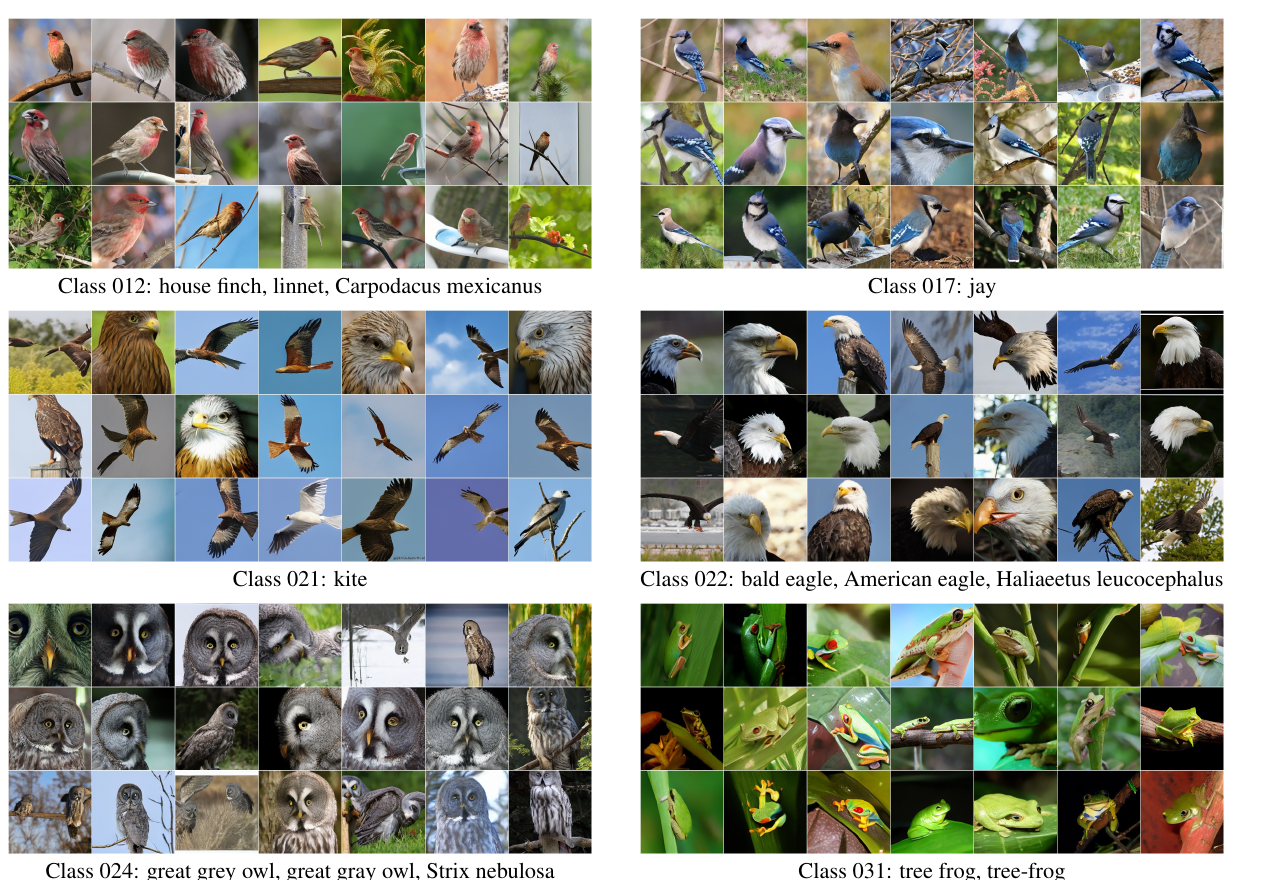
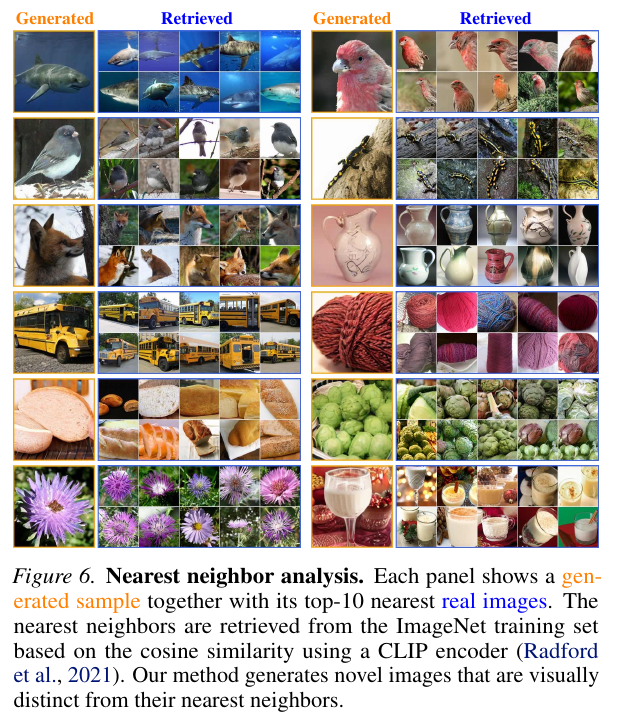
To verify that the generator synthesizes novel images rather than memorizing training examples, Figure 6 retrieves the top-10 nearest neighbors from the ImageNet training set in CLIP embedding space for random 1-NFE generated images, confirming distinct object poses, backgrounds, and lighting structures:
5.3 Visuomotor Robotic Control: 1-NFE Drifting Policy vs. 100-NFE Diffusion Policy (Table 7)
Beyond visual synthesis, the authors test Drifting Models on continuous robotic manipulation benchmarks following the Diffusion Policy protocol (Chi et al., 2023). Here the drifting loss is computed directly in the raw action trajectory space without any feature encoder , replacing the 100-NFE DDPM action head with a 1-NFE Drifting Policy:
| Benchmark Task | Observation Modality | Diffusion Policy (100 NFE) | Drifting Policy (1 NFE) |
|---|---|---|---|
Lift |
State / Visual | 0.98 / 1.00 | 1.00 / 1.00 |
Can |
State / Visual | 0.96 / 0.97 | 0.98 / 0.99 |
ToolHang |
State / Visual | 0.30 / 0.73 | 0.38 / 0.67 |
PushT |
State / Visual | 0.91 / 0.84 | 0.86 / 0.86 |
BlockPush (Multi-Stage) |
State (Phase 1 / Phase 2) | 0.36 / 0.11 | 0.56 / 0.16 |
Kitchen (Multi-Stage) |
State (Phase 1 / 2 / 3 / 4) | 1.00 / 1.00 / 1.00 / 0.99 | 1.00 / 1.00 / 0.99 / 0.96 |
Across both single-stage and multi-stage manipulation tasks, the 1-NFE Drifting Policy matches or outperforms the 100-step Diffusion Policy while cutting action inference calls by 100x.